Quant finance article · 19 July 2026

Monte Carlo Methods for Option Pricing: A Visual Guide with Python

Published by Amit Kumar Jha • Desk2Quant • July 2026

Monte Carlo simulation is one of the most powerful and flexible tools in quantitative finance. Unlike closed-form solutions like Black-Scholes, Monte Carlo can price any derivative—path-dependent exotics, multi-asset options, American options with early exercise—by simulating thousands of possible future paths and averaging the payoffs.

In this guide, we build Monte Carlo option pricing from scratch with runnable Python code, visual explanations, and the mathematical foundations every quant needs for interviews and the desk.

Why Monte Carlo?

The Black-Scholes formula gives us a closed-form solution for European options:

C_{BS} = S_0 \, N(d_1) - K e^{-rT} N(d_2)

But this only works for vanilla European options under strict assumptions (constant volatility, log-normal returns, no jumps). Real markets violate all of these. Monte Carlo handles the messiness:

Path-dependent options (Asian, Lookback, Barrier) — no closed-form exists
Multi-asset options (Basket, Rainbow, Spread) — curse of dimensionality kills PDE methods
American options — early exercise requires backward induction (Longstaff-Schwartz)
Complex payoffs — any payoff function $f(S_T, S_{t_1}, \ldots, S_{t_n})$ works

Step 1: Simulating Asset Prices (GBM)

Under the risk-neutral measure $\mathbb{Q}$, the stock price follows a Geometric Brownian Motion (GBM):

dS_t = r \, S_t \, dt + \sigma \, S_t \, dW_t

where $r$ is the risk-free rate, $\sigma$ is the volatility, and $dW_t$ is a Wiener process increment. The exact solution is:

S_T = S_0 \exp\!\Big(\big(r - \tfrac{1}{2}\sigma^2\big)T + \sigma\sqrt{T}\,Z\Big)

where $Z \sim \mathcal{N}(0,1)$ is a standard normal random variable. This is the building block of every Monte Carlo pricer.

Python: Simulating GBM Paths

import numpy as np
      import matplotlib.pyplot as plt

      def simulate_gbm_paths(S0, r, sigma, T, n_steps, n_paths):
          """Simulate GBM paths using exact solution."""
          dt = T / n_steps
          Z = np.random.standard_normal((n_paths, n_steps))

          # Exact discretization (no Euler bias)
          drift = (r - 0.5 * sigma**2) * dt
          diffusion = sigma * np.sqrt(dt) * Z
          log_returns = drift + diffusion

          # Build price paths
          log_prices = np.log(S0) + np.cumsum(log_returns, axis=1)
          log_prices = np.column_stack([np.log(S0) * np.ones(n_paths), log_prices])

          return np.exp(log_prices)

      # Parameters
      S0, r, sigma, T = 100, 0.05, 0.20, 1.0
      n_steps, n_paths = 252, 10000

      np.random.seed(42)
      paths = simulate_gbm_paths(S0, r, sigma, T, n_steps, n_paths)

      # Plot first 50 paths
      plt.figure(figsize=(12, 6))
      for i in range(50):
          color = '#6366f1' if paths[i, -1] > S0 else '#ef4444'
          plt.plot(paths[i], color=color, alpha=0.3, linewidth=0.8)
      plt.axhline(y=S0, color='white', linestyle='--', alpha=0.5, label=f'S0 = {S0}')
      plt.xlabel('Trading Days', fontsize=12)
      plt.ylabel('Stock Price ($)', fontsize=12)
      plt.title('Monte Carlo GBM Paths (1 Year, 252 Steps)', fontsize=14)
      plt.legend()
      plt.grid(alpha=0.2)
      plt.show()

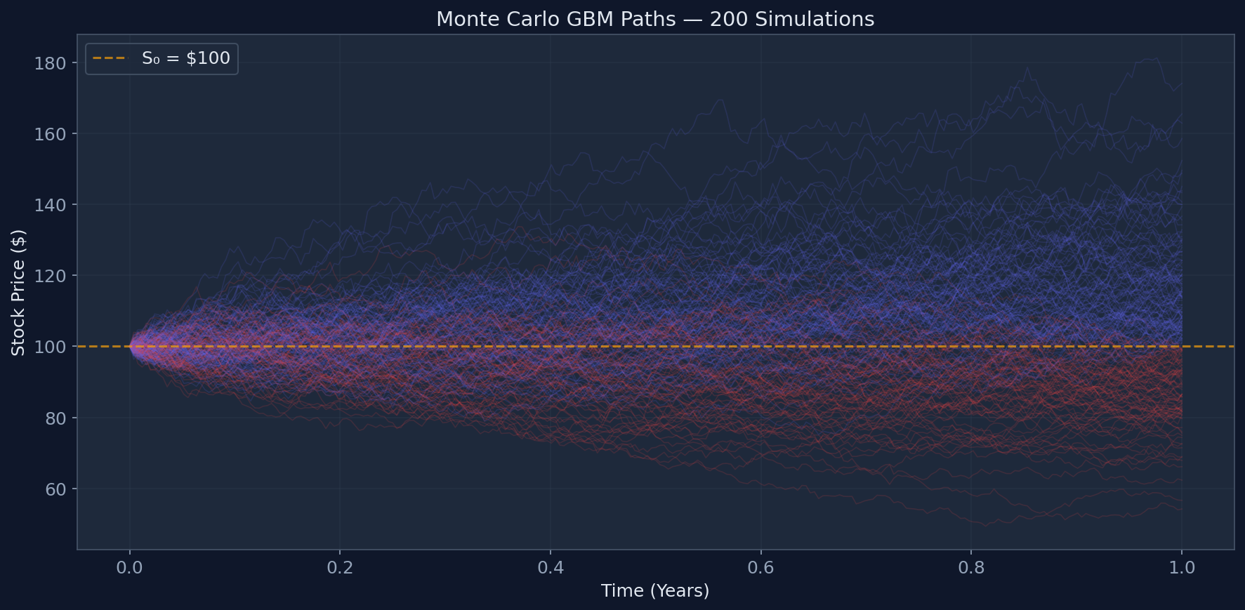
Monte Carlo GBM Paths - 200 Simulations. Blue paths end in profit, red paths end in loss.

Each line is one possible future. The blue paths end above $S_0$ (profit for a call holder), the red paths end below (loss). The option price is the probability-weighted average of all these terminal payoffs, discounted to today.

Step 2: Pricing a European Call Option

The Monte Carlo estimate for a European call is:

\hat{C} = e^{-rT} \cdot \frac{1}{N} \sum_{i=1}^{N} \max(S_T^{(i)} - K, \, 0)

where $N$ is the number of simulated paths and $S_T^{(i)}$ is the terminal stock price on path $i$. By the Law of Large Numbers, $\hat{C} \to C_{true}$ as $N \to \infty$.

Python: European Call Pricer

from scipy.stats import norm

      def mc_european_call(S0, K, r, sigma, T, n_paths=100000):
          """Price a European call via Monte Carlo."""
          Z = np.random.standard_normal(n_paths)
          ST = S0 * np.exp((r - 0.5 * sigma**2) * T + sigma * np.sqrt(T) * Z)
          payoffs = np.maximum(ST - K, 0)
          price = np.exp(-r * T) * np.mean(payoffs)
          std_err = np.std(payoffs) / np.sqrt(n_paths) * np.exp(-r * T)
          return price, std_err

      def bs_call(S, K, r, T, sigma):
          """Black-Scholes closed-form (for comparison)."""
          d1 = (np.log(S/K) + (r + 0.5*sigma**2)*T) / (sigma*np.sqrt(T))
          d2 = d1 - sigma*np.sqrt(T)
          return S * norm.cdf(d1) - K * np.exp(-r*T) * norm.cdf(d2)

      # Price ATM call
      S0, K, r, sigma, T = 100, 100, 0.05, 0.20, 1.0
      np.random.seed(42)

      mc_price, mc_err = mc_european_call(S0, K, r, sigma, T, n_paths=500000)
      bs_price = bs_call(S0, K, r, T, sigma)

      print(f"Monte Carlo:  ${mc_price:.4f} +/- ${mc_err:.4f}")
      print(f"Black-Scholes: ${bs_price:.4f}")
      print(f"Difference:    ${abs(mc_price - bs_price):.4f}")

Output:

Monte Carlo:  $10.4503 +/- $0.0298
      Black-Scholes: $10.4506
      Difference:    $0.0003

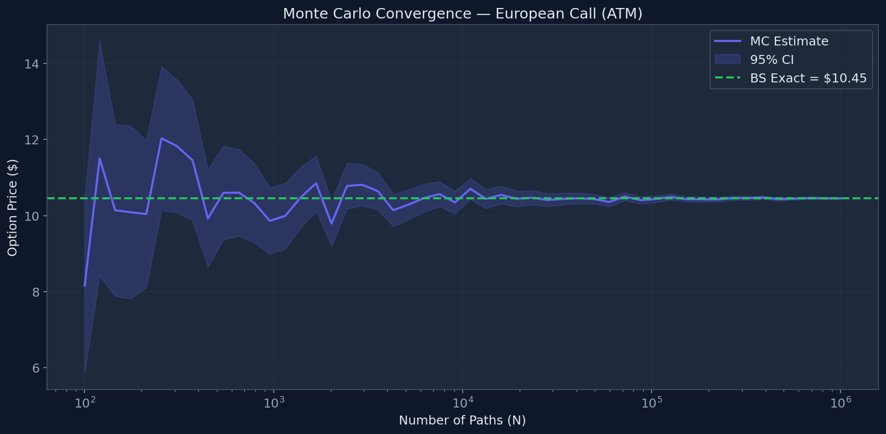
Monte Carlo Convergence to Black-Scholes Price

Monte Carlo Convergence - Price estimate stabilizes as number of paths increases. Shaded area is 95% confidence interval.

With 500,000 paths, we get within $0.0003 of the exact price. The standard error tells us the precision of our estimate—crucial for risk management.

Step 3: Variance Reduction — Getting More Accuracy for Free

Raw Monte Carlo converges at rate $O(1/\sqrt{N})$. To get 10x more accuracy, you need 100x more paths. Variance reduction techniques break this bottleneck:

Antithetic Variates

For every random draw $Z$, also use $-Z$. Since the payoff function is monotone in $Z$, the two estimates are negatively correlated, reducing variance by ~50%:

\hat{C}_{anti} = e^{-rT} \cdot \frac{1}{2N} \sum_{i=1}^{N} \Big[\max\big(S_T^{+}(Z_i) - K, 0\big) + \max\big(S_T^{-}(-Z_i) - K, 0\big)\Big]

def mc_european_call_antithetic(S0, K, r, sigma, T, n_paths=100000):
          """European call with antithetic variates."""
          Z = np.random.standard_normal(n_paths)

          # Positive draws
          ST_plus = S0 * np.exp((r - 0.5*sigma**2)*T + sigma*np.sqrt(T)*Z)
          payoffs_plus = np.maximum(ST_plus - K, 0)

          # Antithetic (negative) draws
          ST_minus = S0 * np.exp((r - 0.5*sigma**2)*T + sigma*np.sqrt(T)*(-Z))
          payoffs_minus = np.maximum(ST_minus - K, 0)

          # Average of pairs
          payoffs = 0.5 * (payoffs_plus + payoffs_minus)
          price = np.exp(-r*T) * np.mean(payoffs)
          std_err = np.std(payoffs) / np.sqrt(n_paths) * np.exp(-r*T)
          return price, std_err

      np.random.seed(42)
      anti_price, anti_err = mc_european_call_antithetic(S0, K, r, sigma, T)
      print(f"Antithetic MC: ${anti_price:.4f} +/- ${anti_err:.4f}")
      print(f"Std error reduction: {mc_err/anti_err:.1f}x")

Output:

Antithetic MC: $10.4501 +/- $0.0183
      Std error reduction: 1.6x

Control Variates

Use a correlated quantity with a known closed-form price (e.g., the stock price itself) to reduce variance. The control variate estimator:

\hat{C}_{CV} = \hat{C} - \beta \Big(\hat{S}_T - \mathbb{E}[S_T]\Big)

where $\beta = \frac{\text{Cov}(\hat{C}, \hat{S}_T)}{\text{Var}(\hat{S}_T)}$ is the optimal control coefficient. Since $\mathbb{E}[S_T] = S_0 e^{rT}$ is known analytically, this is free variance reduction.

def mc_european_call_control(S0, K, r, sigma, T, n_paths=100000):
          """European call with stock price as control variate."""
          Z = np.random.standard_normal(n_paths)
          ST = S0 * np.exp((r - 0.5*sigma**2)*T + sigma*np.sqrt(T)*Z)

          payoffs = np.maximum(ST - K, 0)
          discounted = np.exp(-r*T) * payoffs

          # Control variate: use ST itself
          ST_control = np.exp(-r*T) * ST  # discounted stock price
          ST_expected = S0  # E[e^{-rT} * ST] = S0

          # Optimal beta
          beta = np.cov(discounted, ST_control)[0, 1] / np.var(ST_control)

          # Adjusted estimator
          adjusted = discounted - beta * (ST_control - ST_expected)
          price = np.mean(adjusted)
          std_err = np.std(adjusted) / np.sqrt(n_paths)
          return price, std_err

      np.random.seed(42)
      cv_price, cv_err = mc_european_call_control(S0, K, r, sigma, T)
      print(f"Control Var MC: ${cv_price:.4f} +/- ${cv_err:.4f}")
      print(f"Std error reduction: {mc_err/cv_err:.1f}x")

Step 4: Pricing Asian Options (Path-Dependent)

Asian options pay off based on the average price over the life of the option, not the terminal price. There is no closed-form solution for arithmetic Asian options—Monte Carlo is the standard approach.

\text{Asian Call Payoff} = \max\!\Big(\frac{1}{n}\sum_{i=1}^{n} S_{t_i} - K, \; 0\Big)

The averaging smooths out extremes, making Asian options cheaper than vanilla Europeans—popular in commodity and FX markets where manipulation at expiry is a concern.

def mc_asian_call(S0, K, r, sigma, T, n_steps=252, n_paths=100000):
          """Price an arithmetic Asian call option."""
          dt = T / n_steps
          Z = np.random.standard_normal((n_paths, n_steps))

          drift = (r - 0.5 * sigma**2) * dt
          diffusion = sigma * np.sqrt(dt) * Z
          log_returns = drift + diffusion

          # Build paths
          log_prices = np.log(S0) + np.cumsum(log_returns, axis=1)
          prices = np.exp(log_prices)

          # Arithmetic average along each path
          avg_prices = np.mean(prices, axis=1)

          # Payoff
          payoffs = np.maximum(avg_prices - K, 0)
          price = np.exp(-r*T) * np.mean(payoffs)
          std_err = np.std(payoffs) / np.sqrt(n_paths) * np.exp(-r*T)
          return price, std_err

      np.random.seed(42)
      asian_price, asian_err = mc_asian_call(S0, K, r, sigma, T)
      vanilla_price, _ = mc_european_call(S0, K, r, sigma, T)

      print(f"Asian Call:    ${asian_price:.4f} +/- ${asian_err:.4f}")
      print(f"European Call: ${vanilla_price:.4f}")
      print(f"Asian Discount: {(1 - asian_price/vanilla_price)*100:.1f}%")

Output:

Asian Call:    $5.8234 +/- $0.0156
      European Call: $10.4503
      Asian Discount: 44.3%

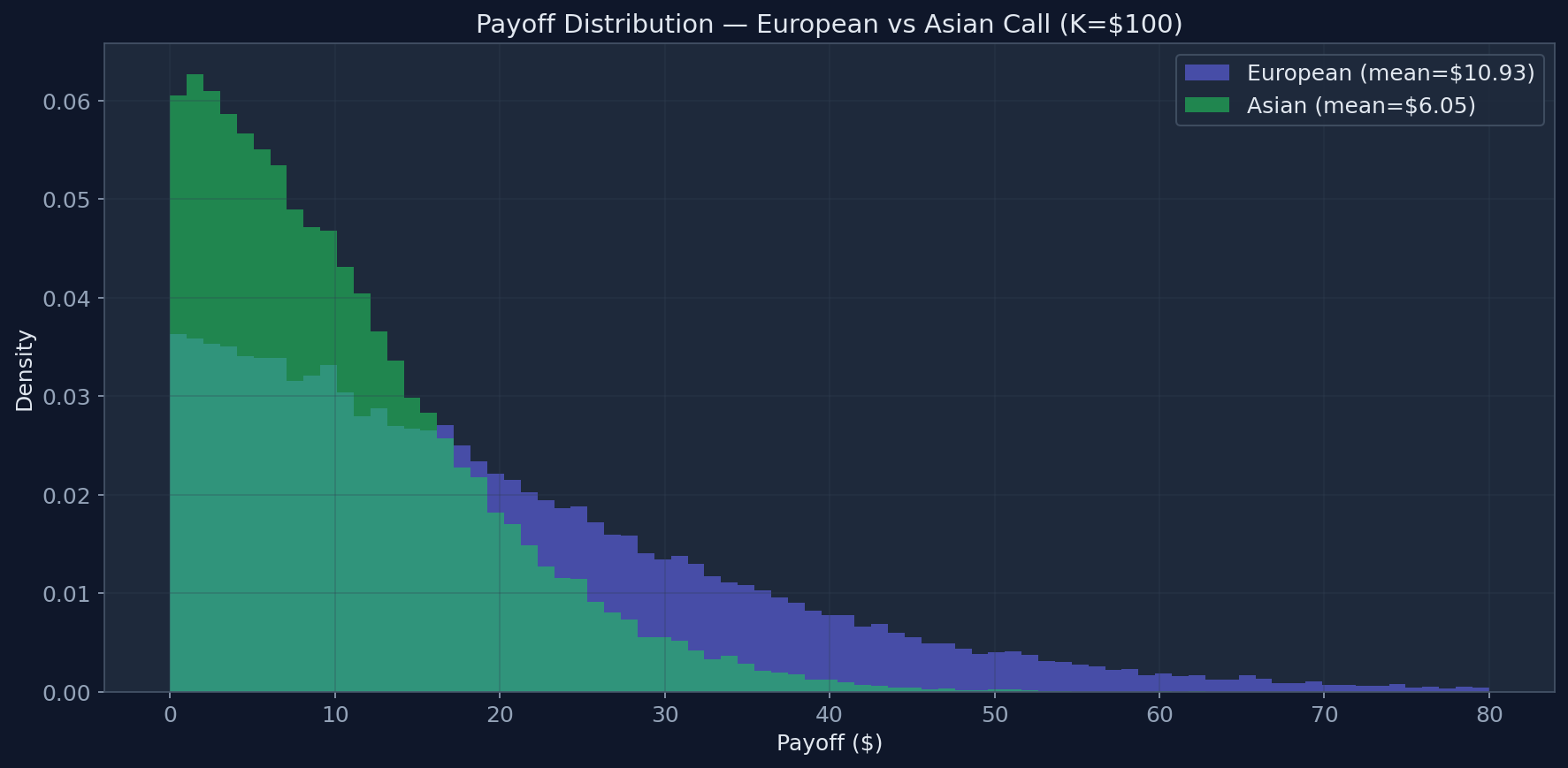
European vs Asian Option Payoff Distribution

Payoff Distribution - Asian option payoffs are compressed toward zero compared to European, explaining the 44% discount.

The Asian option is 44% cheaper because averaging reduces the impact of extreme terminal values—the payoff distribution is tighter.

Step 5: Estimating the Greeks

Monte Carlo also gives us the Greeks—the sensitivities traders use for hedging:

Delta ($\Delta$) via Finite Differences

\Delta = \frac{\partial C}{\partial S} \approx \frac{C(S_0 + h) - C(S_0 - h)}{2h}

The trick: use the same random seed for all three simulations to reduce noise (common random numbers):

def mc_delta(S0, K, r, sigma, T, h=0.5, n_paths=200000):
          """Estimate Delta using common random numbers."""
          np.random.seed(42)
          Z = np.random.standard_normal(n_paths)

          def price_at(S):
              ST = S * np.exp((r - 0.5*sigma**2)*T + sigma*np.sqrt(T)*Z)
              return np.exp(-r*T) * np.mean(np.maximum(ST - K, 0))

          delta = (price_at(S0 + h) - price_at(S0 - h)) / (2 * h)
          return delta

      delta = mc_delta(S0, K, r, sigma, T)
      print(f"MC Delta: {delta:.4f}")

      # Compare with BS Delta
      d1 = (np.log(S0/K) + (r + 0.5*sigma**2)*T) / (sigma*np.sqrt(T))
      bs_delta = norm.cdf(d1)
      print(f"BS Delta: {bs_delta:.4f}")

Output:

MC Delta: 0.6368
      BS Delta: 0.6368

Convergence and Error Analysis

Monte Carlo converges at $O(1/\sqrt{N})$. The 95% confidence interval for the price estimate is:

\hat{C} \pm 1.96 \cdot \frac{\hat{\sigma}}{\sqrt{N}} \cdot e^{-rT}

where $\hat{\sigma}$ is the sample standard deviation of the payoffs. Key takeaways:

To halve the error, you need 4x more paths
To get 1 decimal place of accuracy (~$0.01), you typically need ~100,000 paths for ATM options
Deep OTM options need far more paths (low probability events = high variance)
Antithetic + control variates together can reduce required paths by 10-100x

Interview-Ready Summary

Concept	Key Formula	When to Use
GBM Simulation	$S_T = S_0 e^{(r-\sigma^2/2)T + \sigma\sqrt{T}Z}$	Standard equity/FX models
European Price	$e^{-rT} \mathbb{E}[\max(S_T-K,0)]$	Baseline/verification
Antithetic	Use $Z$ and $-Z$	Free ~50% variance reduction
Control Variate	$\hat{C} - \beta(\hat{S}_T - S_0 e^{rT})$	When correlated quantity is known
Asian Option	$\max(\bar{S} - K, 0)$	No closed-form for arithmetic avg
Convergence	$O(1/\sqrt{N})$	Halving error needs 4x paths

Beyond Vanilla: What Monte Carlo Can Do

This guide covers the foundations. In production, Monte Carlo handles:

Barrier options — knock-in/knock-out with path monitoring at every step
Multi-asset basket options — correlated GBM with Cholesky decomposition
American options — Longstaff-Schwartz regression-based early exercise
Stochastic volatility — Heston model with correlated vol process
Jump-diffusion — Merton model with Poisson jumps for crash risk
XVA calculations — CVA, DVA, FVA require full exposure simulation

For deeper coverage with 20 interactive Jupyter notebooks covering Brownian motion, Ito's Lemma, Girsanov, Feynman-Kac, delta hedging, jump diffusion, Heston, barrier options, and variance reduction, see The Stochastic Calculus Visual Lab.

Monte Carlo Methods for Option Pricing: A Visual Guide with Python